Mobility and Routing in the Soccer Field

This research develops protocols for live monitoring of soccer players during a match. The applet on this page helps visualise inter-connectivity of soccer players of the first-division UNSW soccer club in their game played on 5 Feb 2009. More details are available in the sections below.
Data from the following games can be visualised:

Experimental Setup

With the objective of gaining an understanding of wireless connectivity in a soccer field, both amongst players as well as between players and base-stations, we outfitted all players of the University of New South Wales Football Club (UNSWFC) first-division men's team with wireless monitoring devices. It should be stated that first-division soccer games in Australia are very intense; several of these players go on to become professional footballers playing at the national and international level. We collected data over two trial games held on 28 October 2008 and 5 February 2009. On this page we use the more comprehensive data we were able to collect in the second game, since by then we were able to improve on aspects such as device attachment to the body and base-station placement.

Body Mounting

The body-worn devices we used were the MicaZ motes from Crossbow technologies. These are off-the-shelf devices that are readily available today. We intend to replace these with emerging platforms custom-built for body-area-networking (such as the Toumaz Digital Plaster) as they become available. Though the MicaZ motes were not designed for body-worn applications, they have been used before for body health monitoring, such as in Harvard's Code Blue project, and in our own prior work in profiling the body channel for patients with chronic illnesses. Mounting the motes onto fast-moving athletes such that their motion is not impeded whilst maintaining a good communications link is quite challenging. We tried two positions: arm-mounting using an arm-band, and back-mounting using a chest-strap.

RSSI contours with mote
    mounted on arm 
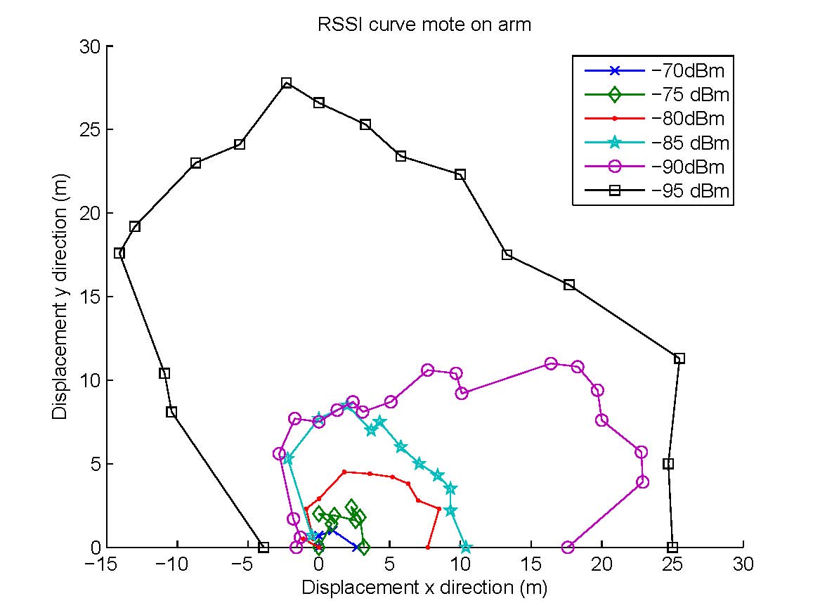
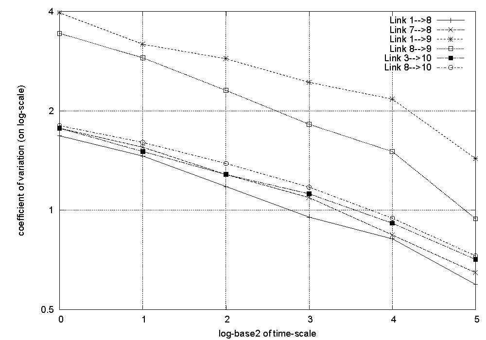
In choosing the preferred mounting position several aspects have to be considered: the attenuation of the wireless signal by the body, the ease and stability of attachment, and the possibility of damage to the device itself. We conducted experiments to profile the propagation of wireless signals around the body in an open field, and show in the Figure above a rough map of the received signal strength indicator (RSSI) at various distances and directions from the body-mounted mote device, which transmits data every second at the highest available power level of 1mW. The person wearing the device is located at (0,0) and is facing north. The Figure shows the RSSI contours when the device is attached to the right arm. Not surprisingly, the reach is much larger to the right (at around 16m the signal fades to below -95dBm) than to the left (signals barely reach beyond 3m), and there is a 5-6m reach to the front and back of the player. By contrast, when the device is mounted on the back, we found that the contours stretch up to 16m to the back, but barely a couple of metres to the front. The smaller wireless ``shadow'' for the arm attachment can be attributed to the smaller cross-section of the body presented to the signal wave. Other reasons also favour an arm-mounted position, such as absence of clothing impediments, and less chance of injury/damage during a fall. These considerations led us to use an arm-mounted position for all our field studies.

Game Layout and Data Collection

RSSI contours with mote
    mounted on arm 
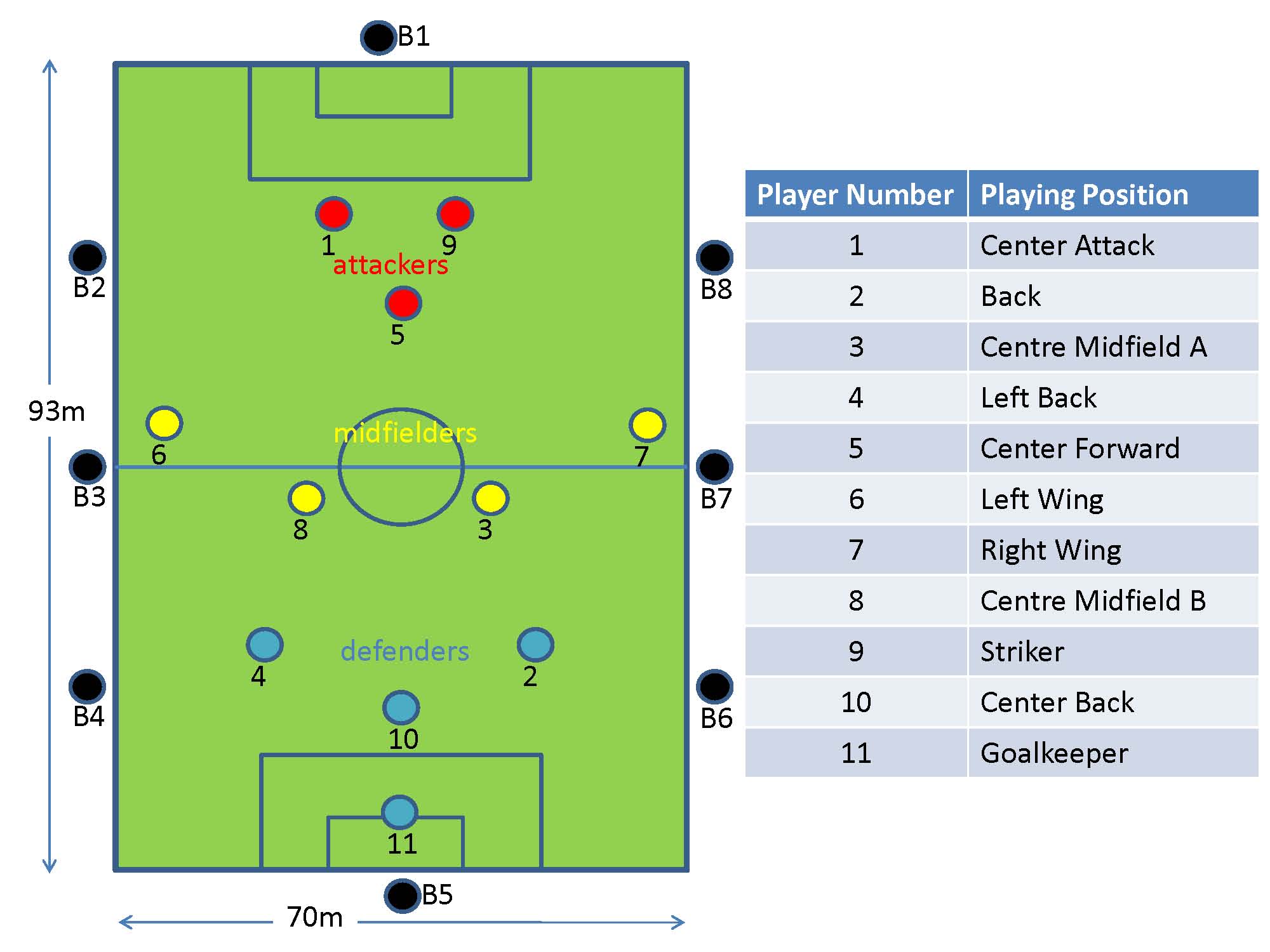
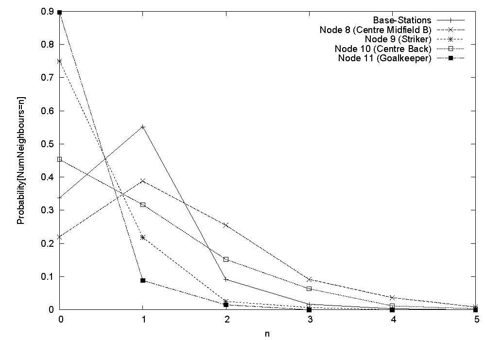
The game was played on a full size field with dimensions 93m x 70m. Each of the 11 players wore a monitoring device on their arm, and 8 base-stations were positioned (at a height of about 1m from the ground) along the sidelines of the playing area. The figure shows the nominal playing positions and associated node identification numbers. Unfortunately the devices worn by players 2 (back) and 4 (left back) were damaged during play and we could not obtain data from them, as was base-station B3 which got hit by the ball. We implemented software on each of the body-worn devices such that it broadcasts, once every second, at the highest available power level of 1mW, a packet containing its unique identifier and a sequence number, during the entire measurement period. All devices (body-worn as well as base-stations) that successfully receive this packet record this event in their on-board memory. As the game proceeds, each node (and base-station) will be cataloguing which other nodes it could hear at each time instant. To prevent collisions in-the-air, each second is divided into 11 slots each of approximate duration 90ms, and each of the 11 body-worn devices is given a unique such slot for transmission every second. Just prior to commencement of the game, the master base-station sends a clock synchronisation message to all nodes, upon receipt of which each node starts recording connectivity data in on-board memory. Data collection stops after 25 minutes, and at the end of the game data from each node is extracted by the master base-station for off-line analysis.

Profiling Player Connectivity

The data collected above tells us how the wireless connectivity between players evolves from second-to-second during the game. In this section we analyse this data and highlight several aspects that are pertinent to the design of routing protocols for real-time extraction of player physiological data. Though we recognise that each soccer game is different and data acquired from repeat trials would undoubtedly yield a different composition of results, our aim is to highlight key common characteristics and trends associated with player connectivity. The Java GUI animation that displays the connectivity data collected for this game should open up as a separate window when you load this page. Though the data was collected for 25 minutes, in this paper we will use only the data collected in the 10 minute interval from 900s to 1500s, since during that period there were no substitutions and no play stoppages. We strongly encourage the reader to observe the Java GUI animation, specifically for the interval 900s-1500s, to get a better feel for the data obtained from the experiment.

Number of Neighbours

Neiughbours for Base-stations (Aggregated) and Node 11 (Goalkeeper) Neighbours for Node 8 (Centre Midfielder B) and Node 9 (Striker)
The figure above shows the time-evolution of the number of neighbours for selected nodes. Specifically, for each selected node, we show at each instant of time, the number of other nodes whose transmissions are successfully received (as we will discuss later links are not always bi-directional). To give a flavour of the diversity we pick players from forward (node9: striker), middle (node 8:centre midfield B), and backward (node 11: goalkeeper) playing positions as well as the base-station (aggregation of all 8 base-stations). Important observations that emerge from these plots are:
Neighbour distribution for base-stations and nodes 8, 9, 10, 11
  • The number of neighbours changes very rapidly, literally from second-to-second, which is not surprising given that soccer players move very fast. Routing therefore has to contend with a highly dynamic topology wherein routes may not persist for long.
  • The average number of neighbours is generally low, indicating that the topology is in general sparse (this can also be confirmed visually in our Java GUI). This is because the range of the body-worn device is small (between 2m and 16m) due to battery current-draw limitations and body attenuation effects, whereas the playing area of the soccer field is large (90m x 73m). The figure on the left plots the probability distribution of the number of neighbours for several nodes, and shows that most of the time a node has 0 or 1 neighbour. Consequently, the number of routing paths available from a node to a base-station is limited.
  • Connectivity varies with playing position: for example, we see that the midfielder (Node 8) has better connectivity (due to prime location in the centre of the field) than the striker or goalkeeper (Node 9 and Node 11), both of whom are more likely to be at the extremes of the field. This is also confirmed in the figure on the left which shows the midfielder is more likely than not to have at least one link at any time, whereas the extreme positions (striker, back, and goalkeeper) have no connectivity very often. Routing can exploit this information to bias its choice of next-hop towards nodes that are more richly-connected on average.
  • Connectivity to the base-stations (put together) is in general quite poor, which implies that multi-hop routing will be essential if real-time delivery of data from players to the base-stations is required.
A detailed study of the impact of the above aspects on routing algorithms for the soccer field is undertaken in our companion submission that is currently under review.

Encounter Duration and Inter-Encounter Time

Another metric that is known to have an important bearing on the route-selection algorithm in mobile ad-hoc networks is the inter-encounter time (also known as inter-meeting or inter-contact time) between nodes. Most prior studies have relied on exponentially distributed inter-encounter times for tractable anaysis of routing performance; however, recent studies have shown that non-exponential behaviour can lead to unbounded routing delays. To see which model best fits the soccer field environment, in the figures below we show the distribution of the inter-encounter time amongst all pairs of nodes, as well as between all transmitters and a specific receiver 8 (the centre midfield B, chosen for its rich connectivity), as obtained from our experimental data.
Distribution of inter-encounter time on log-linear scale Distribution of inter-encounter time on log-log scale
The figure on the left shows the Complementary Cumulative Distribution Function (CCDF) of the inter-encounter time on log-linear scale. The non-linear nature of the curve, particularly at time scales ranging from 1 to 200 seconds, indicates that the inter-encounter delays do not follow an exponential distribution at such time-scales. In the figure on the right we therefore depict the inter-encounter time on log-log scale, and notice that in the range of 10-100 seconds the inter-encounter delay curve (over all pairs of nodes) is roughly linear, indicative of power-law behaviour in that range. The power-law exponent in this region is estimated at around &alpha &asymp 1.6. Though earlier works have analytically evaluated that &alpha < 2 leads to unbounded routing delays, it does so by extrapolating the inter-encounter delay tail to infinity as a power-law. Our experimental data shows that the curve flattens out (on log-linear scale) beyond around 200 seconds, and in this region inter-encounters are better modelled as exponential. This combination of power-law and exponential behaviour is consistent with reported mixtures seen in inter-meeting times for regular human activity. Moreover, routing delays for such a mixture are bounded; indeed our companion work develops routing algorithms for the soccer field that can route the player data to base-stations within acceptable delays.
Distribution of encounter duration (log-linear scale) Log-log plot of link coefficient-of-variation
Another aspect in which the soccer field environment departs from typical mobile ad-hoc networks is the length of time for which two nodes are in continuous contact with each other for exchanging routing messages and data packets. The figure on the left above shows the CCDF of the duration for which encounters last (on log-linear scale) over all pairs of nodes and with node 8 (centre midfielder B) as receiver. It is seen that encounters are in general very short (over 90% of encounters lasts no more than 4 seconds), and their duration falls exponentially (the curves are near-linear on log-linear scale). A routing algorithm cannot therefore assume sufficient contact time with a neighbour in order to be able to forward all its stored messages, or indeed even sufficient time for bidirectional communication with the neighbour.
To characterise the encounter and inter-encounter distributions and their auto-correlations in a succinct way (which we later employ in our model below), we borrow a technique used for the analysis of long-range dependent (LRD) traffic. Considering a link between a pair of nodes, at a given time step, we use a 1 to depict presence of the link and 0 its absence. For this link, we therefore have from our experimental data a time-sequence of 0s and 1s. We consider this sequence in blocks of 2s samples, for given s, and for this resulting sequence we compute the mean, variance, and coefficient-of-variation &beta(s) (in effect these metrics are computed at time-scale 2s). Log-log plots of &beta(s) versus s are routinely used in the literature to depict self-similarity and to estimate the corresponding Hurst parameter H &isin [0.5,1). In the figure on the right above we show such a plot for several links (we picked two links each from centre, forward, and backward playing positions), and observe that the curves can be approximated as straight-lines with slope -(1-H), yielding a Hurst parameter H &asymp 0.75. This single-parameter captures in a succinct way the link auto-correlations, and will be used in the connectivity model we develop in a later section.

Link Correlations

Unlike many mobile ad-hoc networks in which we can reasonably assume that users move independently, in a soccer game we would expect player movements to have significant correlations. For example, when the team is attacking the opponent's goal, several players in the forward and midfield positions can be expected to move towards the opponent's goal simultaneously, and conversely when the home goal is being attacked the defenders and midfielders will likely fall back towards the home goal to protect it. This leads to correlations amongst links, and knowledge of such correlations can be exploited by routing to improve delay performance: for example, in a two-hop routing scheme in which packets go from source s to the base-station B via an intermediate node, the source could bias its choice of intermediate hop towards nodes i that have high correlation between the links s &rarr i and i &rarr B so as to reduce end-to-end delays. Correlations are computed as follows: if xt is a binary variable that is 1 or 0 depending on whether link x is present or absent at time step t, then the cross-correlation at time lag k between two links x and y is computed as:
&rhoxy(k) = 1/n &sumt=1n-k (xt-x)(yt+k-y) / &sigmax &sigmay, for k=0, ± 1, ± 2, ...
where n is the number of sample points, x is the estimated mean and &sigmax the estimated standard deviation of x.
correlation between links 3 &rarr 8 and 10 &rarr 8 correlation between links 1 &rarr 8 and 10 &rarr 8
In the figure above on the left we show the correlation between node 3's (centre midfield A) and node 10's (centre back) links to node 8 (the centre midfield B) for lags in the range [-20,20] seconds. Two things are noteworthy from this plot: (a) the correlations are positive, meaning that when node 3 is close to node 8, node 10 is also likely to be close to node 8; this suggests nodes 3 and 10 move in a co-ordinated way quite often, and (b) the correlations are high (>0.2) for lag close to 0, and decay rapidly as the lag moves away from 0. This is not surprising, because the fast nature of the game implies that the locations of the players can vary significantly from one minute to the next, making them nearly independent. In the figure on the right we show the correlation between node 1's (centre attack) and node 10's (centre back) with node 8 (centre midfield B). This time we notice that the correlations are predominantly negative (<-0.2 for lags close to 0), which is understandable: when the team is attacking, the midfielder is more likely to be close to the striker and far from the defender, while the converse is true when the team is defending their own goal. Again we notice that the anti-correlations decay with time due to the rapid movement of players in the game.
Correlations depicted via inter-connections Correlations shown as a matrix
Having seen specific examples of correlated and anti-correlated links, let us now examine how pervasive the correlations are amongst all links. We have data from 9 transmitters (as stated earlier the devices on two players got damaged and the data was lost) and 10 receivers (9 players and a ``virtual'' base-station which aggregates the data from all base-stations), giving us a total of 81 possible uni-directional links. During the 10 minute measurement period, 60 of these links had sufficient (at least 10) packet receptions to be statistically significant, and so we compute pair-wise cross-correlations for these 60 links. To eliminate random chance of correlated values, we also estimate the P-value (used for statistical hypothesis testing) for each pair, and only retain those that are statistically significant (i.e. have P &le 0.05). To help the reader visualise the correlations, we place the 60 links as nodes on a circle in the left on the left above and draw a line between two nodes if they have significant correlation: blue lines depict positive correlation while red lines depict negative correlation, and the higher the correlation (or anti-correlation), the thicker the line. Also, links have been ordered on the circle so that the two directions of the link are adjacent to each other (so that correlations between the two directions of a link do not clutter the plot). We see that often links to a given player (say player 8, the centre midfielder B) can have strong correlations with each other, but some links with distinct end-points can also be correlated (for example, link 1 &rarr 10 is correlated with links 8 &rarr 3, 5 &rarr 3 and 7 &rarr 3, indicating that when an attacker 1 is close to a defender 10, many players are likely to be huddled closer to the ball, and hence more likely to be connected to a midfield player such as 3). To give an idea of how widespread the correlations are, in the figure on the right we show the elements of the 60x60 correlation matrix that are significant. The matrix is seen to be relatively sparse, which suggests that determining the entire matrix (needed as input to our model presented next) may not be as onerous as one may think.